בינה מאלכותית RB14-16 : ניבוי סדרות ורצפים עם בינה מלאכותית LSTM
:part 1
complex things start simple ….. LSTM
1,2,3,4,….?
|
1 2 3 4 5 6 7 8 9 10 11 12 13 14 15 16 17 18 19 20 21 22 23 24 25 26 27 28 29 30 31 32 33 |
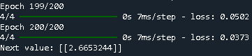
import numpy as np from tensorflow.keras.models import Sequential from tensorflow.keras.layers import Dense, LSTM, Input # Dataset 1–100 data = np.array(range(1, 101)) # Sliding windows X, y = [], [] for i in range(len(data)-3): X.append(data[i:i+3]) y.append(data[i+3]) X = np.array(X) y = np.array(y) # Reshape for LSTM [samples, timesteps, features] X = X.reshape((X.shape[0], X.shape[1], 1)) # Build model (Input layer first) model = Sequential() model.add(Input(shape=(3,1))) # define input shape here model.add(LSTM(50, activation='relu')) model.add(Dense(1)) model.compile(optimizer='adam', loss='mse') # Train model.fit(X, y, epochs=200, verbose=1) # Test test_input = np.array([1,2,3]).reshape((1,3,1)) print("Next value:", model.predict(test_input, verbose=0)) |
LSTM is used. I’ll explain every object, function, and parameter.
how the program works
1) Imports
-
numpy as np: numerical arrays and reshaping. -
Sequential: a Keras model type where layers are stacked in order. -
Dense: a fully connected (feed-forward) layer. -
LSTM: Long Short-Term Memory layer (a recurrent layer for sequences). -
Input: explicitly declares the input tensor shape.
2) Build a simple dataset (integers 1..100)
-
Creates
data = [1, 2, 3, ..., 100]as a NumPy array.
3) Create sliding windows (supervised sequences)
-
For each position
i, take a 3-number window as input and the next number as the target. -
Example: when
i=0,X[0]=[1,2,3],y[0]=4; wheni=1,X[1]=[2,3,4],y[1]=5, etc. -
Because the window length is 3, the last usable start is at index
len(data)-4, so there arelen(data)-3 = 97samples.
Convert to arrays:
4) Reshape X for LSTM: [samples, timesteps, features]
-
LSTM expects 3D input:
(batch, timesteps, features_per_timestep). -
Here:
samples=97,timesteps=3(the window length),features=1(each timestep is a single scalar). -
Final
X.shape == (97, 3, 1).
5) Define the model
Layer by layer:
-
Input(shape=(3,1))-
Declares that each training example is a sequence of length 3, with 1 feature per time step.
-
-
LSTM(50, activation='relu')-
LSTM is a gated recurrent unit that processes the 3 timesteps in order, maintaining an internal memory (cell state) to model temporal patterns.
-
units=50: the size of the LSTM hidden state (number of LSTM cells). -
activation='relu': the activation applied to the candidate/output (default istanh; here it’s changed to ReLU). -
Important default parameters (not shown but used):
-
recurrent_activation='sigmoid'for the input/forget/output gates. -
return_sequences=False(outputs only the last time step’s output vector of length 50). -
dropout=0.0,recurrent_dropout=0.0by default.
-
Parameter count (informative):
For LSTM, params =4 * units * (units + input_dim + 1)
Here:units=50,input_dim=1→4 * 50 * (50 + 1 + 1) = 4 * 50 * 52 = 10,400. -
-
Dense(1)-
Fully connected layer mapping the 50-dim output from LSTM to a single scalar prediction (the next number).
-
Params:
50*1 + 1 = 51.
-
-
Total trainable parameters:
10,400 + 51 = 10,451.
6) Compile the model (training configuration)
-
optimizer='adam': adaptive gradient method (good default). -
loss='mse': mean squared error for regression (predicting a real number).
7) Train
-
X:(97,3,1)inputs;y:(97,)targets. -
epochs=200: the whole dataset is iterated 200 times. -
verbose=1: prints a progress bar and per-epoch loss. -
Default
batch_size=32: with 97 samples, batches are typically sizes 32, 32, 33 per epoch.
What the LSTM learns:
Given sequences like [n, n+1, n+2] → target (n+3), it learns the rule “next value ≈ previous value + 1” (i.e., a simple linear progression) from examples 1..100.
8) Test inference
-
test_inputshape(1,3,1)matches the model’s expected input. -
The LSTM processes the three timesteps
[1,2,3]and outputs a scalar close to4.0. -
verbose=0silences prediction logs.
What “using an LSTM” means here
-
Across the 3 timesteps, the LSTM updates its hidden state and cell state using input/forget/output gates, allowing it to model temporal dependencies.
-
Even though the sequence is very short (length 3), the LSTM treats it as a time series, not just a static 3-vector. It “reads” values in order and uses its memory mechanism to summarize them before the Dense layer maps that summary to the next value.
Notes and typical improvements (optional)
-
For time-series regression,
activation='tanh'in LSTM is common;relucan work but may be less stable for some data. -
Normalizing the data (e.g., scaling 1..100 to 0..1) often improves training.
-
Use a proper train/validation split to check generalization.
-
Longer windows (more timesteps) help when the next value depends on more history.
That’s it: the code frames next-step prediction as sequence modeling, prepares 3-step windows, trains an LSTM to map each window to its next value, and demonstrates prediction on [1,2,3] → ~4.
|
1 2 3 4 5 6 7 8 9 10 11 12 13 14 15 16 17 18 19 20 21 22 23 24 25 26 27 28 29 30 31 32 33 |
import numpy as np from tensorflow.keras.models import Sequential from tensorflow.keras.layers import Dense, LSTM, Input # Dataset 1–100 data = np.array(range(1, 101)) # Sliding windows X, y = [], [] for i in range(len(data)-3): X.append(data[i:i+3]) y.append(data[i+3]) X = np.array(X) y = np.array(y) # Reshape for LSTM [samples, timesteps, features] X = X.reshape((X.shape[0], X.shape[1], 1)) # Build model (Input layer first) model = Sequential() model.add(Input(shape=(3,1))) # define input shape here model.add(LSTM(50, activation='relu')) model.add(Dense(1)) model.compile(optimizer='adam', loss='mse') # Train model.fit(X, y, epochs=200, verbose=1) # Test test_input = np.array([1,2,3]).reshape((1,3,1)) print("Next value:", model.predict(test_input, verbose=0)) |
part 2 :
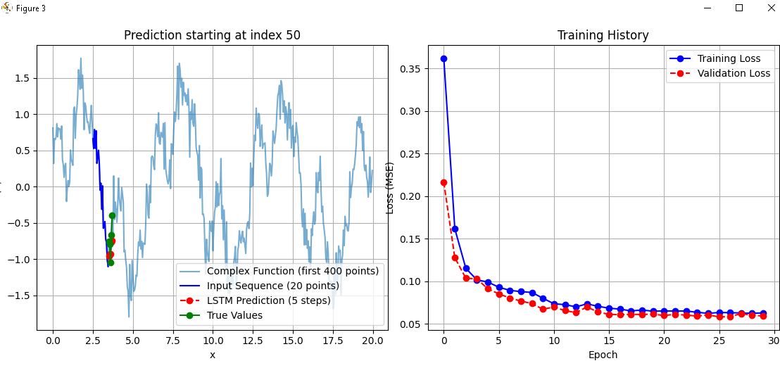
Let try far more complex sequence to predict
|
1 2 3 4 5 6 7 8 9 10 11 12 13 14 15 16 17 18 19 20 21 22 23 24 25 26 27 28 29 30 31 32 33 34 35 36 37 38 39 40 41 42 43 44 45 46 47 48 49 50 51 52 53 54 55 56 57 58 59 60 61 62 63 64 65 66 67 68 69 70 71 72 73 74 75 76 77 78 79 80 81 82 83 84 85 86 87 88 89 90 91 92 93 94 95 96 97 98 99 100 101 102 103 104 105 106 107 108 109 110 111 112 113 114 115 116 117 118 119 120 121 122 123 124 125 126 127 128 129 130 131 132 133 134 135 136 137 138 139 140 141 142 143 |
# -*- coding: utf-8 -*- """ Created on Wed Sep 24 20:17:56 2025 @author: dev66 """ # -*- coding: utf-8 -*- """ Created on Wed Sep 24 20:09:38 2025 @author: dev66 Description: ------------ This program builds and trains an LSTM model to predict the next 5 points of a more complex periodic function (sine + cosine + sine mix + noise). It then visualizes: - The first part of the function (default: 400 points) - The input sequence window - The predicted vs. true next 5 points - Training history (loss curves) """ import numpy as np import matplotlib.pyplot as plt from tensorflow.keras.models import Sequential from tensorflow.keras.layers import LSTM, Dense, Input # ========================================================== # 1. Generate dataset function (with noise parameter) # ========================================================== def generate_function(x, noise_level=0.0): """ Generate a complex function with optional Gaussian noise. f(x) = sin(x) + 0.5*cos(3x) + 0.3*sin(5x) + noise Parameters ---------- x : np.ndarray Input values. noise_level : float Standard deviation of Gaussian noise to add. Returns ------- np.ndarray Generated data with noise. """ base = np.sin(x) + 0.5*np.cos(3*x) + 0.3*np.sin(5*x) noise = noise_level * np.random.randn(len(x)) return base + noise # Generate data x = np.linspace(0, 100, 2000) # 2000 points data = generate_function(x, noise_level=0.2) # adjust noise_level here # ========================================================== # 2. Prepare training sequences # ========================================================== window_size = 20 # input: 20 past points predict_ahead = 5 # output: 5 future points X, y = [], [] for i in range(len(data) - window_size - predict_ahead): X.append(data[i:i+window_size]) y.append(data[i+window_size:i+window_size+predict_ahead]) X = np.array(X) y = np.array(y) # Reshape for LSTM: (samples, timesteps, features) X = X.reshape((X.shape[0], X.shape[1], 1)) # ========================================================== # 3. Build the LSTM model # ========================================================== model = Sequential() model.add(Input(shape=(window_size, 1))) model.add(LSTM(64, activation='tanh')) # 64 units for more capacity model.add(Dense(predict_ahead)) # output = 5 points model.compile(optimizer='adam', loss='mse') # ========================================================== # 4. Train the model # ========================================================== history = model.fit(X, y, epochs=30, verbose=1, validation_split=0.2) # ========================================================== # 5. Flexible prediction function # ========================================================== def predict_from_index(model, data, x, start_index, window_size, predict_ahead): """ Use a trained model to predict 'predict_ahead' values starting from a given index in the dataset. Plots results and training history. """ start_seq = data[start_index:start_index + window_size] test_input = start_seq.reshape((1, window_size, 1)) prediction = model.predict(test_input, verbose=0).flatten() true_future = data[start_index+window_size:start_index+window_size+predict_ahead] # ======== Plot ======== plt.figure(figsize=(15,5)) # (a) Function (first 400 points) + input + prediction plt.subplot(1,2,1) plt.plot(x[:400], data[:400], label="Complex Function (first 400 points)", alpha=0.6) plt.plot(x[start_index:start_index+window_size], start_seq, 'b', label="Input Sequence (20 points)") plt.plot(x[start_index+window_size:start_index+window_size+predict_ahead], prediction, 'ro--', label="LSTM Prediction (5 steps)") plt.plot(x[start_index+window_size:start_index+window_size+predict_ahead], true_future, 'g-o', label="True Values") plt.title(f"Prediction starting at index {start_index}") plt.xlabel("x") plt.ylabel("f(x)") plt.legend() plt.grid(True) # (b) Training history plt.subplot(1,2,2) plt.plot(history.history['loss'], 'b-o', label="Training Loss") plt.plot(history.history['val_loss'], 'r--o', label="Validation Loss") plt.title("Training History") plt.xlabel("Epoch") plt.ylabel("Loss (MSE)") plt.legend() plt.grid(True) plt.tight_layout() plt.show() return prediction, true_future # ========================================================== # 6. Example usage # ========================================================== start_index = 50 # try values <= 180 so it's visible in first 200 points prediction, true_future = predict_from_index(model, data, x, start_index, window_size, predict_ahead) print(f"\nPrediction from index {start_index+window_size} " f"to {start_index+window_size+predict_ahead-1}:") print("Predicted:", prediction) print("True :", true_future) |
Block 1: Imports and Setup
We start by importing the required libraries:
numpy is used for arrays and numbers, matplotlib.pyplot (optional) is for visualization, and tensorflow.keras provides the tools to build and train the LSTM model.
Block 2: Generate Dataset Function
Next, we define the function that builds our dataset:
This function creates a signal that combines sine and cosine waves, then adds Gaussian noise. The noise_level parameter controls how much randomness is introduced.
Block 3: Generate Data
We then generate 2000 data points:
Here, x is evenly spaced between 0 and 100. The function is applied to these points, with a small noise level of 0.2.
Block 4: Prepare Training Sequences
To prepare the dataset for training, we use sliding windows:
Each training input (X) contains the previous 20 values, and the corresponding output (y) contains the next 5 values. Finally, X is reshaped into the 3D format required by LSTMs: samples, timesteps, features.
Block 5: Build the LSTM Model
We now construct the model:
The model takes 20 values as input, passes them through an LSTM layer with 64 units, and then outputs 5 predicted values. It uses the Adam optimizer and mean squared error as the loss function.
Block 6: Train the Model
Training the model is done with:
The model is trained for 30 epochs. Twenty percent of the dataset is reserved for validation.
Block 7: Prediction Function
We define a function to make predictions starting at any given index:
This function reshapes the last 20 values into the correct format, predicts the next 5 values, and also retrieves the true 5 values for comparison.
Block 8: Example Usage
Finally, we test the model by predicting future values:
Here, we choose start_index = 50. The model predicts the next 5 values after this point, and we print both the predicted values and the actual true values.