בינה מלאכותית RB108-6 : בינה מלאכותית – איך נוירון לומד

חלק א :

שימו לב !!!

בהסבר זה לפעמים אני מראה חישוב על ערך X אחד בלבד – זה עלמנת שהכל יהיה ברור וקל במציאות יש לחשב את כל הערכים עבור פונקציה LOST MSE

x = [-3, -2, -1, 0, 1, 2, 3]

y = [-5, -3, -1, 1, 3, 5, 7]

those are the true values :y = [-5, -3, -1, 1, 3, 5, 7]

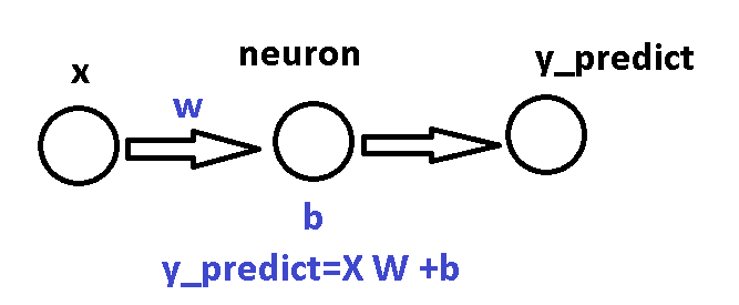
1) The Neuron Model

The neuron predicts:

Starting values:

2) Forward Pass (Prediction)

For each x:

x	y_true	y_predict
-3	-5	-3
-2	-3	-2
-1	-1	-1
0	1	0
1	3	1
2	5	2
3	7	3

3).Error , lost Function

we start w=1,b=0

`y_true = w * x + b`

`y_predict = w * x + b`

x	y_true	y_predict = 1·x + 0	error = y_predict – y_true	loss = (y_true – y_predict)²
-3	-5	-3	+2	4
-2	-3	-2	+1	1
-1	-1	-1	0	0
0	1	0	-1	1
1	3	1	-2	4
2	5	2	-3	9
3	7	3	-4	16

Totals for Step 3

Sum of errors:

$2 + 1 + 0 - 1 - 2 - 3 - 4 = - 7$

Sum of loss values:

$4 + 1 + 0 + 1 + 4 + 9 + 16 = 35$

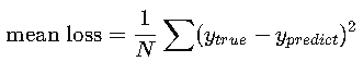
Mean Loss (The Value Used for Learning)

The Mean Loss is:

$samples\text{mean loss} = \frac{\text{sum of all losses}}{\text{number of samples}}$

In our case:

Total loss = 35
Number of samples = 7

So:

MSE (mean squared error) = cost function = Error loss

3.1 Why we use the Loss and not the Error

Example:

Loss converts both to:

So the neuron learns how big the mistake is, not just the sign.

Raw error cancels out:

Loss does NOT cancel out → always correct for learning.

4.Gradients for a Single Neuron

We will calculate the gradients for w , b

Step 1 — Start With the Loss Function

For one training sample:

This is the loss the neuron wants to minimize.

Step 2 — Substitute the Neuron Output

The neuron predicts:

Substitute into the loss:

Derivative With Respect to w

dL/dw = 2x (y_predict – y_true)

We use the chain rule.

A) Define inner function

Then:

B) Outer derivative

C) Inner derivative

u = y_true – w*x – b

Derivative with respect to w:

D) Combine (Chain Rule)

Rewrite using y_predict = w*x + b:

4) Gradients are computed from the loss – Gradients for a Single Neuron

dL/dw = 2x (y_predict – y_true)
dL/db = 2 (y_predict – y_true)

Derivative With Respect to w

We use the chain rule.

A) Define inner function

Then:

B) Outer derivative

C) Inner derivative

u = y_true – w*x – b

Derivative with respect to w:

D) Combine (Chain Rule)

Rewrite using y_predict = w*x + b:

Derivative With Respect to b (Step-by-Step)

We again use the chain rule.

A) Define the inner function

We define:

The loss is:

B) Outer derivative

Derivative of L = u² with respect to u:

C) Inner derivative (with respect to b)

Write u again:

Derivative of u with respect to b:

Because only “–b” depends on b.

D) Combine (Chain Rule)

Now multiply the inner and outer derivatives:

Substitute:

Rewrite Using y_predict

Since:

Then:

Substitute into the formula:

Why We Don’t Solve With Derivative = 0 (Except for One Neuron)

1) For a single neuron (like your example):

This is a simple line.

We can take the derivative of the loss, set it to 0, and solve for the exact best:

This works because the loss surface is a perfect parabola (a simple bowl shape).

2) But for many neurons (real neural networks):

When you add:

more neurons
more layers
activation functions (ReLU, sigmoid)
millions of parameters

The loss surface becomes:

twisted
curved
full of valleys and hills
impossible to solve with algebra

You cannot write equations like:

for millions of nonlinear parameters.

There is no formula that gives all w and b directly.

Gradient Descent (Step-by-Step With Example)

שימו לב !!!

בהסבר זה אני מראה חישוב על ערך X אחד בלבד – זה עלמנת שהכל יהיה ברור וקל במציאות יש לחשב את כל הערכים עבור פונקציה LOST MSE

Gradient Descent is the action step where the neuron actually updates
the weight w and the bias b to reduce the loss.

We use:

Where:

η (eta) = learning rate
dL/dw, dL/db = gradients
w_old, b_old = values before update
w_new, b_new = values after update

Example Setup (single x , not all dataset for keep it simple )

We use this data point for simplicity:

Prediction:

Error:

Gradients:

Now we perform Gradient Descent.

Epoch 1 — Update w and b

Update weight

Update bias

End of Epoch 1:

The neuron has learned a little.

Epoch 2 — Repeat With New w and b

1) Forward Pass

2) Error

3) Gradients

4) Update Step

End of Epoch 2:

The neuron is now closer to the true pattern.

Final Summary (Easy to Understand)

Epoch	w	b
Start	1.00	0.00
1	1.20	0.20
2	1.36	0.36

Gradient Descent is the step that actually updates w and b.
The gradient tells the direction.
Gradient Descent moves the weights in that direction.

Gradients Also Require ALL Data (Full Batch Training)

Before we use the full dataset, let’s start with the basic gradient formulas for a single sample:

These formulas work when you use one training example at a time.

But real training uses all samples together to compute one global update.

Using ALL Data: Full Batch Gradients

If you have N samples:

Then the total loss is:

And the Mean Squared Error (MSE) is:

This is the value we minimize.

Single-Sample Loss and Gradient

For one sample:

Gradient:

This is correct only for one point.

Full-Batch Gradient Descent — Epoch 1 and Epoch 2 …. (with updated w and b)

We use your dataset:

Start values:

EPOCH 1 — FULL STEPS

1) Forward Pass (All Samples)

x	y_true	*y_predict (1x + 0)**	error	error²
-3	-5	-3	+2	4
-2	-3	-2	+1	1
-1	-1	-1	0	0
0	1	0	-1	1
1	3	1	-2	4
2	5	2	-3	9
3	7	3	-4	16

Total Loss = 35

MSE = 35 / 7 = 5

2) Compute Full-Batch Gradients

Gradient for w

Formula:

**Compute Σ[x * error]:**

Apply formula:

Gradient for b

Formula:

Compute Σ error:

Now:

3) UPDATE w AND b (Epoch 1)

Update rule:

Update w

Update b

End of Epoch 1

EPOCH 2 — FULL STEPS

Now use:

1) Forward Pass (Using New w, b)

Compute predictions:

x	y_true	y_predict	error	error²
-3	-5	-4.1	+0.9	0.81
-2	-3	-2.7	+0.3	0.09
-1	-1	-1.3	-0.3	0.09
0	1	0.1	-0.9	0.81
1	3	1.5	-1.5	2.25
2	5	2.9	-2.1	4.41
3	7	4.3	-2.7	7.29

Total Loss = 15.75

MSE = 15.75 / 7 ≈ 2.25

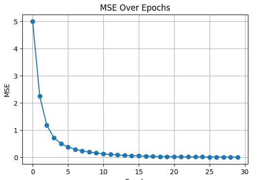
Loss dropped from 5 → 2.25 — learning works.

2) Gradients (Full Batch)

**Σ x * error**

dL/dw:

Σ error

dL/db:

3) UPDATE w AND b (Epoch 2)

Update w:

Update b:

End of Epoch 2

Final Summary Table

Epoch	w	b	MSE
1	1.40	0.10	5.00
2	1.64	0.19	2.25

As training continues, the neuron moves toward the true values:

# ============================================================
# SIMPLE LINEAR NEURON LEARNING WITH GRADIENT DESCENT
# NOW WITH ROUND(…, 4) FOR CLEAR PRINTED VALUES
# ============================================================

import numpy as np
import matplotlib.pyplot as plt

# -----------------------------
# 1) Dataset (your exact data)
# -----------------------------
x = np.array([-3, -2, -1, 0, 1, 2, 3], dtype=float)
y_true = np.array([-5, -3, -1, 1, 3, 5, 7], dtype=float)

# -----------------------------
# 2) Initial parameters
# -----------------------------
w = 1.0
b = 0.0
lr = 0.05
epochs = 30

mse_history = []

print("INITIAL CONDITIONS:")
print(f"w = {w}, b = {b}\n")

# ============================================================
# TRAINING LOOP — FULL BATCH GRADIENT DESCENT
# ============================================================
for epoch in range(1, epochs + 1):

    # 1) Forward pass
    y_pred = w * x + b
    error = y_pred - y_true
    mse = np.mean(error ** 2)

    # 2) Full batch gradients
    dLdw = (2 / len(x)) * np.sum(x * error)
    dLdb = (2 / len(x)) * np.sum(error)

    # Store for plot
    mse_history.append(mse)

    # 3) PRINT ALL DETAILS (rounded)
    print("-----------------------------------------------------")
    print(f"Epoch {epoch}")
    print("-----------------------------------------------------")
    print("Predictions:", np.round(y_pred, 4))
    print("Errors:     ", np.round(error, 4))
    print(f"MSE (error loss): {round(mse, 4)}")

    print(f"dL/dw: {round(dLdw, 4)}")
    print(f"dL/db: {round(dLdb, 4)}")

    # 4) Update rules
    w = w - lr * dLdw
    b = b - lr * dLdb

    print(f"Updated w = {round(w, 4)}")
    print(f"Updated b = {round(b, 4)}\n")

# ============================================================
# PLOT MSE
# ============================================================
plt.figure(figsize=(6, 4))
plt.plot(mse_history, marker='o')
plt.title("MSE Over Epochs")
plt.xlabel("Epoch")
plt.ylabel("MSE")
plt.grid(True)
plt.show()

# ============================================================

# SIMPLE LINEAR NEURON LEARNING WITH GRADIENT DESCENT

# NOW WITH ROUND(…, 4) FOR CLEAR PRINTED VALUES

# ============================================================

import numpy as np

import matplotlib.pyplot as plt

# -----------------------------

# 1) Dataset (your exact data)

# -----------------------------

x = np.array([-3, -2, -1, 0, 1, 2, 3], dtype=float)

y_true = np.array([-5, -3, -1, 1, 3, 5, 7], dtype=float)

# -----------------------------

# 2) Initial parameters

# -----------------------------

w = 1.0

b = 0.0

lr = 0.05

epochs = 30

mse_history = []

print("INITIAL CONDITIONS:")

print(f"w = {w}, b = {b}\n")

# ============================================================

# TRAINING LOOP — FULL BATCH GRADIENT DESCENT

# ============================================================

for epoch in range(1, epochs + 1):

# 1) Forward pass

y_pred = w * x + b

error = y_pred - y_true

mse = np.mean(error ** 2)

# 2) Full batch gradients

dLdw = (2 / len(x)) * np.sum(x * error)

dLdb = (2 / len(x)) * np.sum(error)

# Store for plot

mse_history.append(mse)

# 3) PRINT ALL DETAILS (rounded)

print("-----------------------------------------------------")

print(f"Epoch {epoch}")

print("-----------------------------------------------------")

print("Predictions:", np.round(y_pred, 4))

print("Errors: ", np.round(error, 4))

print(f"MSE (error loss): {round(mse, 4)}")

print(f"dL/dw: {round(dLdw, 4)}")

print(f"dL/db: {round(dLdb, 4)}")

# 4) Update rules

w = w - lr * dLdw

b = b - lr * dLdb

print(f"Updated w = {round(w, 4)}")

print(f"Updated b = {round(b, 4)}\n")

# ============================================================

# PLOT MSE

# ============================================================

plt.figure(figsize=(6, 4))

plt.plot(mse_history, marker='o')

plt.title("MSE Over Epochs")

plt.xlabel("Epoch")

plt.ylabel("MSE")

plt.grid(True)

plt.show()

Activation function

Why Didn’t We Add an Activation Function in Our Example?

Because in our example you were teaching:

a single neuron
simple linear regression
with the goal to learn

$y = 2 x + 1$

In this case, you must NOT add an activation function,
because any activation will break the linearity and prevent the neuron from learning the correct straight line.

When Do We Actually Add Activation Functions?

Activation functions are needed only when the problem is non-linear.

We add them when we have:

✔ Deep neural networks
✔ Non-linear tasks
✔ Classification problems
✔ XOR (classic non-linear problem)
✔ Images
✔ Audio
✔ Text
✔ Any pattern that is not a straight line

חלק ב

ניתוח קובץ אקסל :

תרגיל כיתה א – שימוש בבינה מלאכותית לניתוח תוצאות של קובץ אקסל CHATGPT

נתח את קובץ האקסל exp1 יבא אותו ל chatGpt

1.1 בקשו גרף קורציות מפת חום בין הטבאלות איפה ניראה שיש קורלציות Correlation Map Between Columns

בקשו הבינה המלאכותית – לנתח את הנתונים

2.1 כמה קבוצות של רמה בחשבון יש ?

2.2 מה הפרמטרים שמשפעים על כל קבוצה – הנמוכה 0 , והקבוצה 3 הגבוהה ביותר

2.3 איזה עצה היית נותן שיש לאנשים הכנסה נמוכה ואין כסף למורים פרטים עבור שילהם שלהם יהיו טובים בחשבון ?

3.3 לפי הנתונים האלה האם לכל ילד שנולד יש הזדמנות טובה להיות טוב במטמתיקה ?

נתח את קובץ האקסל exp1 יבא אותו ל chatGpt

1.1 בקשו גרף קורלציות מפת חום בין הטבלאות איפה ניראה שיש קורלציות Correlation Map Between Columns

בקשו הבינה המלאכותית – לנתח את הנתונים

2.1 כמה קבוצות של רמה בחשבון יש ?

2.2 מה הפרמטרים שמשפעים על כל קבוצה – הנמוכה 0 , והקבוצה 3 הגבוהה ביותר

2.3 איזה עצה היית נותן שיש לאנשים הכנסה נמוכה ואין כסף למורים פרטים עבור שלהם שלהם יהיו טובים בחשבון ?

3.3 לפי הנתונים האלה האם לכל ילד שנולד יש הזדמנות טובה להיות טוב במתמטיקה ?

שיווק מוצר בעזרת בינה מלאכותית – תרגיל כיתה

יצירת וידאו : מטקסט – שיווק מוצר עם בינה מלאכותית

יצירת וידאו : מתמונה וטקסט – שיווק מוצר עם בינה מלאכותית

2.תרגיל כיתה : פיתוח מוצר בעזרת בינה מלאוכתית

1.1 התחלקו לצוות של 2 או 3 אנשים , וחשבו על מוצר המצאה שתרצו לשווק או לייצר – מה סוג המוצר ? לשוק דובר השפה האנגלית

2. בידקו בעזרת בינה מלאוכתית מי המתחרים , מה טווח מחירים בקשו קישורים למוצרים בתחום

2.1 איזה אתרים אפשרי לקבל מידע על מתחרים עבור הנמוצר בשוק באתרים חפש בעזרת בינה מלאוכתית : אמזון אייבי ועליקספרסס

3. שאל את הבינה מלאוכתית , באיזה 50 אתרים בעולם ניתן וממולץ למכור את המוצר ומה השלבים ?

הכנת חומר שיווקי עבור המוצר .

4. הכינו תמונה של המוצר טקסט , הסבר קצר , ותאור מפורט על המוצר

4.1 מה יהיה מחיר עלות להערכת הבינה מלאכותית ומה מחיר מכירה ?

5. בעזרת תוכנת canva צרו דמות AVATAR שמתארת את המוצר , תמונה של המוצר בשפה האנגלית

6. צרו את הסרטון והעלו אותו ל YOUTUBE

בינה מלאכותית RB108-6 : בינה מלאכותית – איך נוירון לומד

חלק א :

x = [-3, -2, -1, 0, 1, 2, 3]

y = [-5, -3, -1, 1, 3, 5, 7]

1) The Neuron Model

2) Forward Pass (Prediction)

3).Error , lost Function

y_true = w * x + b

y_predict = w * x + b

Totals for Step 3

Sum of errors:

Sum of loss values:

Mean Loss (The Value Used for Learning)

So:

mean loss=357=5

MSE (mean squared error) = cost function = Error loss

3.1 Why we use the Loss and not the Error

Example:

4.Gradients for a Single Neuron

We will calculate the gradients for w , b

Step 1 — Start With the Loss Function

Step 2 — Substitute the Neuron Output

Derivative With Respect to w

A) Define inner function

B) Outer derivative

C) Inner derivative

D) Combine (Chain Rule)

dL/dw = 2x (y_predict – y_true) dL/db = 2 (y_predict – y_true)

Derivative With Respect to w

A) Define inner function

B) Outer derivative

C) Inner derivative

D) Combine (Chain Rule)

Derivative With Respect to b (Step-by-Step)

A) Define the inner function

B) Outer derivative

C) Inner derivative (with respect to b)

D) Combine (Chain Rule)

Rewrite Using y_predict

Why We Don’t Solve With Derivative = 0 (Except for One Neuron)

1) For a single neuron (like your example):

y=wx+b

This is a simple line.

We can take the derivative of the loss, set it to 0, and solve for the exact best:

w=2,b=1

This works because the loss surface is a perfect parabola (a simple bowl shape).

2) But for many neurons (real neural networks):

When you add:

more neurons

more layers

activation functions (ReLU, sigmoid)

millions of parameters

The loss surface becomes:

twisted

curved

full of valleys and hills

impossible to solve with algebra

You cannot write equations like:

∂L∂w=0

for millions of nonlinear parameters.

There is no formula that gives all w and b directly.

Gradient Descent (Step-by-Step With Example)

Example Setup (single x , not all dataset for keep it simple )

Epoch 1 — Update w and b

Update weight

Update bias

End of Epoch 1:

Epoch 2 — Repeat With New w and b

1) Forward Pass

2) Error

3) Gradients

4) Update Step

End of Epoch 2:

Final Summary (Easy to Understand)

Gradients Also Require ALL Data (Full Batch Training)

Using ALL Data: Full Batch Gradients

Single-Sample Loss and Gradient

Full-Batch Gradient Descent — Epoch 1 and Epoch 2 …. (with updated w and b)

We use your dataset:

Start values:

`y_true = w * x + b`

`y_predict = w * x + b`

dL/dw = 2x (y_predict – y_true)
dL/db = 2 (y_predict – y_true)

**Compute Σ[x * error]:**

**Σ x * error**