בינה מאלכותית RB14-18 : מהו PASCAL VOC 2007 – benchmark dataset and competition
PASCAL VOC 2007 is a labeled dataset of 20 everyday object classes, with bounding boxes, used for training and evaluating object detection models.
PASCAL VOC stands for Pattern Analysis, Statistical Modelling and Computational Learning – Visual Object Classes.
It was a benchmark dataset and competition created in 2007 to push forward object detection and recognition.
Researchers trained models on its images and compared results using a standard evaluation metric (mAP)
Why It’s Important
-
It became a standard benchmark for early detection models like YOLOv1, Faster R-CNN, SSD.
-
It is smaller and simpler than today’s COCO dataset, so it’s still used for teaching, prototyping, and quick experiments.
What is PASCAL VOC 2007?
2. What’s Inside the Dataset?
-
Images: about 9,963 images of real-world scenes.
-
Objects: about 24,000 labeled objects.
-
Classes: 20 categories, including:
-
Person
-
Animals (dog, cat, bird, horse, sheep, cow)
-
Vehicles (car, bus, motorbike, bicycle, train, aeroplane, boat)
-
Household items (chair, sofa, tv/monitor, dining table, bottle, potted plant)
-
3. Annotations (Bounding Boxes)
Each image comes with an annotation file that tells:
-
What object is present (e.g., “dog”).
-
Where it is located (bounding box: top-left corner and bottom-right corner pixel coordinates).
|
1 2 3 4 5 6 7 8 9 |
<object> <name>dog</name> <bndbox> <xmin>50</xmin> <ymin>60</ymin> <xmax>200</xmax> <ymax>220</ymax> </bndbox> </object> |
This means there is a dog in the rectangle defined by those pixel coordinates
Perfect, let’s build Step 1: A Python program that will:
-
Download the PASCAL VOC 2007 dataset
-
List the labels (20 classes)
-
Print the annotation structure (so you see how labels are stored)
-
Show a few images with their bounding boxes
|
1 |
pip install matplotlib pillow |
hose libraries are built into Python’s standard library and do not require pip install:
-
os → already in Python, for file system paths.
-
tarfile → already in Python, for extracting
.tararchives. -
urllib.request → already in Python, for downloading files.
-
xml.etree.ElementTree → already in Python, for parsing XML annotation files.
The only things you need to install manually (via pip) are external libraries that are not in the standard library:
-
matplotlib → plotting (drawing images + bounding boxes).
-
pillow (PIL) → image loading and manipulation.
And since patches comes from matplotlib (from matplotlib import patches), installing matplotlib is enough.
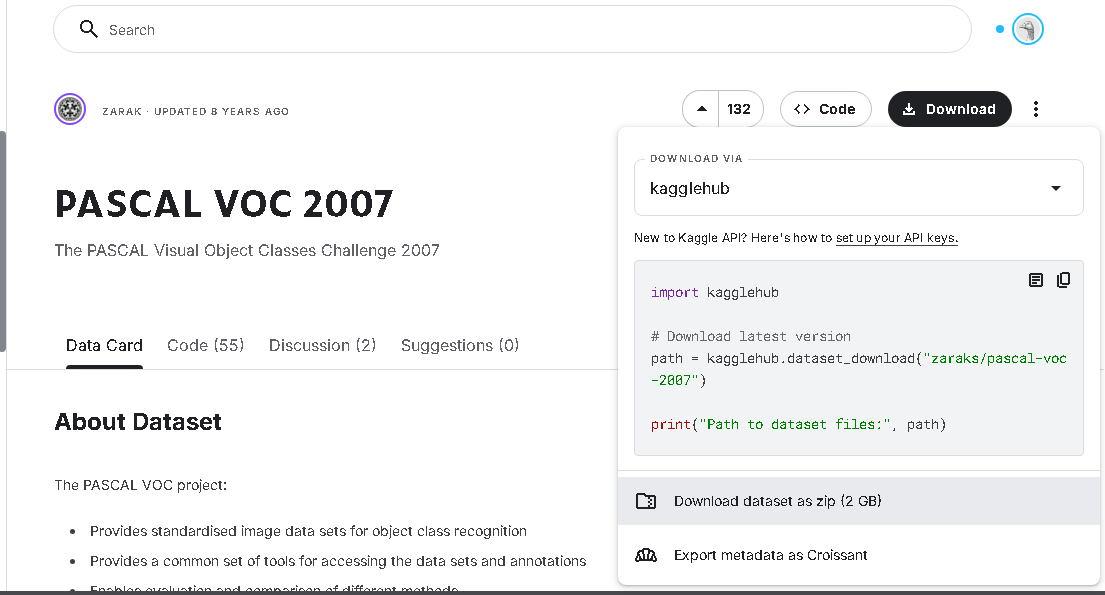
https://www.kaggle.com/datasets/zaraks/pascal-voc-2007
|
1 2 3 4 5 6 7 8 9 10 11 12 13 14 15 16 17 18 19 20 21 22 23 24 25 |
PASCAL-VOC-2007/ PASCAL_VOC/ PASCAL_VOC/ VOCtest_06-Nov-2007/ VOCdevkit/ VOC2007/ Annotations/ ImageSets/ Layout/ Main/ Segmentation/ JPEGImages/ SegmentationClass/ SegmentationObject/ VOCtrainval_06-Nov-2007/ VOCdevkit/ VOC2007/ Annotations/ ImageSets/ Layout/ Main/ Segmentation/ JPEGImages/ SegmentationClass/ SegmentationObject/ |
point to:
-
Train/Val set →
D:\temp\PASCAL-VOC-2007\VOCtrainval_06-Nov-2007\VOCdevkit\VOC2007 -
Test set →
D:\temp\PASCAL-VOC-2007\VOCtest_06-Nov-2007\VOCdevkit\VOC2007
|
1 2 3 4 5 6 7 8 9 10 11 12 13 14 15 16 17 18 19 20 21 22 23 24 25 26 27 28 29 30 31 32 33 34 35 36 37 38 39 40 41 42 43 44 45 46 47 48 49 50 51 52 53 54 55 56 57 58 59 60 61 62 63 64 65 66 67 68 69 70 71 72 73 74 75 76 77 78 79 80 81 82 83 84 85 86 87 88 89 90 91 92 93 94 95 96 |
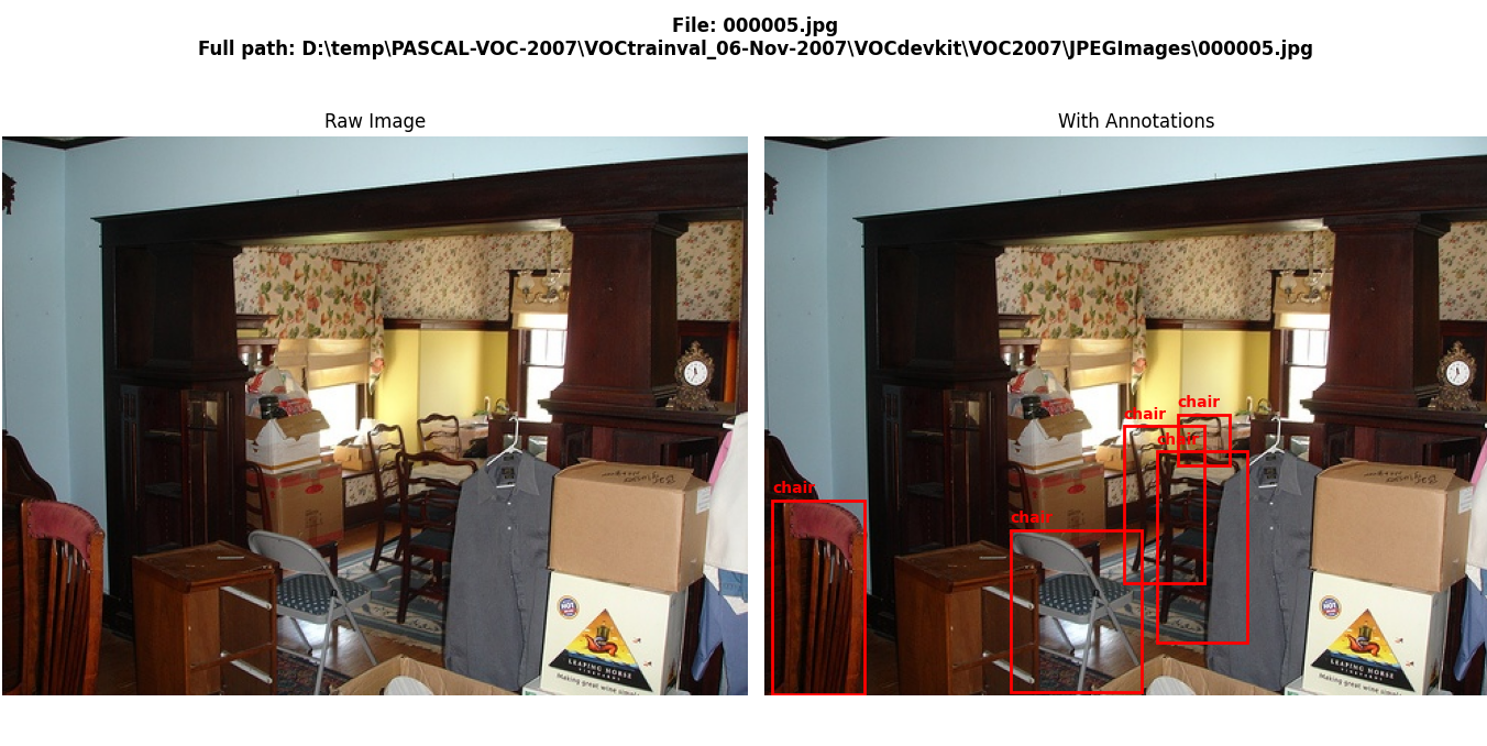
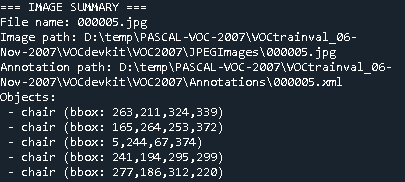
import os import xml.etree.ElementTree as ET import matplotlib.pyplot as plt import matplotlib.patches as patches from PIL import Image import random # ========================================================== # 1. Dataset paths # ========================================================== voc_trainval = r"D:\temp\PASCAL-VOC-2007\VOCtrainval_06-Nov-2007\VOCdevkit\VOC2007" voc_test = r"D:\temp\PASCAL-VOC-2007\VOCtest_06-Nov-2007\VOCdevkit\VOC2007" # Choose split voc_dir = voc_trainval ann_dir = os.path.join(voc_dir, "Annotations") img_dir = os.path.join(voc_dir, "JPEGImages") # ========================================================== # 2. Parse annotation file # ========================================================== def parse_annotation(xml_file): tree = ET.parse(xml_file) root = tree.getroot() objects = [] for obj in root.findall("object"): cls = obj.find("name").text bbox = obj.find("bndbox") xmin = int(bbox.find("xmin").text) ymin = int(bbox.find("ymin").text) xmax = int(bbox.find("xmax").text) ymax = int(bbox.find("ymax").text) objects.append((cls, xmin, ymin, xmax, ymax)) return objects # ========================================================== # 3. Show image side by side (raw vs annotated) # ========================================================== def show_side_by_side(img_file, objects): img = Image.open(img_file) # Create two subplots: raw + annotated fig, (ax1, ax2) = plt.subplots(1, 2, figsize=(14, 7)) fig.suptitle(f"File: {os.path.basename(img_file)}\nFull path: {img_file}", fontsize=12, weight="bold") # Left: raw image ax1.imshow(img) ax1.set_title("Raw Image") ax1.axis("off") # Right: annotated image ax2.imshow(img) for (cls, xmin, ymin, xmax, ymax) in objects: rect = patches.Rectangle((xmin, ymin), xmax - xmin, ymax - ymin, linewidth=2, edgecolor='red', facecolor='none') ax2.add_patch(rect) ax2.text(xmin, ymin - 5, cls, color='red', fontsize=10, weight="bold") ax2.set_title("With Annotations") ax2.axis("off") plt.tight_layout() plt.show() # ========================================================== # 4. Switch: random or manual # ========================================================== mode = "manual" # "random" or "manual" if mode == "random": example_ann = random.choice(os.listdir(ann_dir)) elif mode == "manual": file_number = "000005" # <-- choose manually here example_ann = file_number + ".xml" else: raise ValueError("Mode must be 'random' or 'manual'") example_ann_path = os.path.join(ann_dir, example_ann) objects = parse_annotation(example_ann_path) example_img = os.path.join(img_dir, example_ann.replace(".xml", ".jpg")) # ========================================================== # 5. Print summary and show side by side # ========================================================== print("=== IMAGE SUMMARY ===") print("File name:", os.path.basename(example_img)) print("Image path:", example_img) print("Annotation path:", example_ann_path) print("Objects:") for obj in objects: cls, xmin, ymin, xmax, ymax = obj print(f" - {cls} (bbox: {xmin},{ymin},{xmax},{ymax})") # Show raw + annotated images side by side show_side_by_side(example_img, objects) |
the script so that in addition to writing everything into the text file, it also prints a dataset summary to the console at the end. This will include:
-
Total number of images processed
-
Total number of objects found
-
Average objects per image
-
A per-class breakdown (how many times each category appears across the dataset)
Full Program with Console Summary
|
1 2 3 4 5 6 7 8 9 10 11 12 13 14 15 16 17 18 19 20 21 22 23 24 25 26 27 28 29 30 31 32 33 34 35 36 37 38 39 40 41 42 43 44 45 46 47 48 49 50 51 52 53 54 55 56 57 58 59 60 61 62 63 64 65 66 67 68 69 70 71 72 73 74 75 76 77 |
import os import xml.etree.ElementTree as ET from collections import Counter # ========================================================== # 1. Dataset path # ========================================================== voc_trainval = r"D:\temp\PASCAL-VOC-2007\VOCtrainval_06-Nov-2007\VOCdevkit\VOC2007" voc_dir = voc_trainval # or switch to voc_test ann_dir = os.path.join(voc_dir, "Annotations") img_dir = os.path.join(voc_dir, "JPEGImages") # ========================================================== # 2. Parse annotation XML # ========================================================== def parse_annotation(xml_file): tree = ET.parse(xml_file) root = tree.getroot() objects = [] for obj in root.findall("object"): cls = obj.find("name").text bbox = obj.find("bndbox") xmin = int(bbox.find("xmin").text) ymin = int(bbox.find("ymin").text) xmax = int(bbox.find("xmax").text) ymax = int(bbox.find("ymax").text) objects.append((cls, xmin, ymin, xmax, ymax)) return objects # ========================================================== # 3. Process all files # ========================================================== annotations = [f for f in os.listdir(ann_dir) if f.endswith(".xml")] print(f"Start reading {len(annotations)} annotation files...") summary_file = "voc2007_summary.txt" total_objects = 0 class_counter = Counter() with open(summary_file, "w", encoding="utf-8") as f: for idx, ann in enumerate(annotations, start=1): ann_path = os.path.join(ann_dir, ann) img_path = os.path.join(img_dir, ann.replace(".xml", ".jpg")) objects = parse_annotation(ann_path) total_objects += len(objects) for cls, xmin, ymin, xmax, ymax in objects: class_counter[cls] += 1 # Write detailed info to file f.write(f"File name: {os.path.basename(img_path)}\n") f.write(f"Image path: {img_path}\n") f.write(f"Annotation path: {ann_path}\n") f.write("Objects:\n") for cls, xmin, ymin, xmax, ymax in objects: f.write(f" - {cls} (bbox: {xmin},{ymin},{xmax},{ymax})\n") f.write("\n" + "="*50 + "\n\n") # Print progress every 10 files if idx % 10 == 0: print(".", end="", flush=True) # ========================================================== # 4. Print summary to console # ========================================================== print("\n\n=== DATASET SUMMARY ===") print(f"Total files processed: {len(annotations)}") print(f"Total objects found: {total_objects}") print(f"Average objects per image: {total_objects / len(annotations):.2f}") print("\nObjects per class:") for cls, count in class_counter.most_common(): print(f" - {cls}: {count}") print(f"\n✅ Detailed summary written to {summary_file}") |
verything we’ve built so far is about reading and analyzing the PASCAL VOC 2007 dataset (images + XML annotations).
That’s the preparation stage:
-
Making sure the dataset is accessible.
-
Parsing the XML annotations.
-
Summarizing what’s inside.
So far, no AI model is involved — we are just checking the dataset
IoU = Intersection over Union
Definition:
IoU measures how much the predicted bounding box overlaps with the ground-truth bounding box.
Formula:
IoU=Area of OverlapArea of UnionIoU = \frac{\text{Area of Overlap}}{\text{Area of Union}}
-
Area of Overlap = the common region between the predicted box and the real box.
-
Area of Union = total area covered by both boxes together.
So IoU ranges from 0 to 1:
-
IoU = 1 → Perfect match (boxes identical).
-
IoU = 0 → No overlap at all.
-
IoU = 0.5 → Boxes overlap by 50%.
In PASCAL VOC 2007, a detection is considered correct (TP) only if:
IoU≥0.5IoU \geq 0.5
If IoU < 0.5 → the box does not overlap enough → it’s treated as a False Positive (FP).
This means:
-
Your predicted box must cover at least half of the true box area to count as correct
✅ True Positive (TP) Example
Ground truth box (dog):
x = 50, y = 50, width = 100, height = 100
Predicted box (dog):
x = 55, y = 55, width = 100, height = 100
Step 1: Compute Overlap (Intersection)
-
The overlapping region width = 95 (since 100 − 5)
-
The overlapping region height = 95
-
Overlap area = 95 × 95 = 9025
Step 2: Compute Union
Union=Area(pred)+Area(gt)−Overlap\text{Union} = \text{Area(pred)} + \text{Area(gt)} – \text{Overlap}
→ 100×100+100×100−9025=10975100×100 + 100×100 – 9025 = 10975
Step 3: Compute IoU
IoU=902510975≈0.822IoU = \frac{9025}{10975} ≈ 0.822
Interpretation:
IoU = 0.82 ≥ 0.5 → this detection matches the ground truth well,
so it is counted as a True Positive (TP).
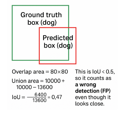
❌ False Positive (FP) Example (yours)
Ground truth box (dog):
x = 50, y = 50, width = 100, height = 100
Predicted box (dog):
x = 60, y = 60, width = 100, height = 100
→ Overlap = 80×80 = 6400
→ Union = 13600
→ IoU = 6400 / 13600 = 0.47
IoU < 0.5 → this detection is too far off, counted as False Positive (FP).
🔎 Summary:
| Case | IoU | Result | Meaning |
|---|---|---|---|
| TP Example | 0.82 | ✅ TP | Good overlap (correct detection) |
| FP Example | 0.47 | ❌ FP | Poor overlap (wrong detection) |
Mean Average Precision (mAP)
mAP measures how well an object detector finds and localizes objects across all categories.
High mAP = fewer false positives + fewer missed detections.
-
Compute AP for each class separately.
-
Take the mean across all classes:
mAP=1N∑c=1NAPcmAP = \frac{1}{N}\sum_{c=1}^N AP_c
where NN = number of classes.
Example:
-
AP(car) = 0.70
-
AP(person) = 0.80
-
AP(dog) = 0.60
→ mAP = (0.70 + 0.80 + 0.60) / 3 = 0.70
Confusion Matrix Terms
Every prediction you make can be categorized into one of four cases:
1. TP = True Positive
-
The model predicts an object, and it is correct.
-
Example: The model predicts a “dog” box, and there really is a dog in that location (IoU ≥ 0.5 with ground truth).
2. FP = False Positive
-
The model predicts an object, but it is wrong.
-
Example: The model predicts a “dog” in the image, but there is no dog there (or IoU < 0.5).
-
Another case: The class is wrong (predicted “cat” but it’s a “dog”).
3. FN = False Negative
-
The model misses a real object.
-
Example: There is a dog in the image, but the model does not detect it at all.
4. TN = True Negative (rarely used in detection)
-
The model correctly says “nothing here.”
-
In image classification it’s common, but in object detection with large search space, TN is not usually counted.
🔹 How They Work Together
-
Precision = TP / (TP + FP)
→ “Of all boxes I predicted, how many were correct?” -
Recall = TP / (TP + FN)
→ “Of all real objects, how many did I find?”
🔎 Example
Imagine an image has 2 dogs:
-
Your model predicts 3 boxes:
-
2 match the dogs (good → TP=2)
-
1 is wrong (bad → FP=1)
-
-
But it misses 0 dogs (FN=0).
So:
-
TP = 2
-
FP = 1
-
FN = 0
Precision = 2 / (2+1) = 0.67
Recall = 2 / (2+0) = 1.0
✅ In short:
-
TP = correct detection
-
FP = false alarm
-
FN = missed object
How to Interpret
-
mPA is given as a percentage (0–100)
-
Example:
-
16 mPA→ 16% average pixel accuracy (very poor model, most pixels misclassified). -
79 mPA→ 79% average pixel accuracy (quite strong model, most pixels correct). -
21 mPA→ 21% average pixel accuracy (weak, better than random but still low).
-
In YOLOv8, the metric labeled mAP50 (and sometimes displayed as mPA depending on your environment or UI) represents mean Average Precision at IoU 0.5, following the PASCAL VOC evaluation standard.
Here’s a precise breakdown of what YOLOv8 reports:
1. Key Metrics YOLOv8 Prints During Training
When you train or validate a model, you’ll see metrics like:
-
Box(P) → Precision = TP / (TP + FP)
-
Box(R) → Recall = TP / (TP + FN)
-
mAP50 → mean Average Precision at IoU = 0.5
-
Same as VOC 2007 style (looser overlap requirement).
-
-
mAP50-95 → mean AP averaged over IoU thresholds 0.5 → 0.95 (COCO-style).
If you see mPA = 79, that is mAP50 = 0.79 — meaning your model correctly detects objects about 79% of the time at IoU ≥ 0.5.
2. How YOLOv8 Calculates mAP
-
It checks every prediction against ground truth using IoU (Intersection over Union).
-
A prediction counts as True Positive (TP) if IoU ≥ 0.5 and the class matches.
-
Otherwise, it’s a False Positive (FP).
-
Using all predictions, YOLOv8 builds Precision–Recall curves per class.
-
The area under each curve = AP (Average Precision) for that class.
-
The mean across all classes = mAP.
3. Typical YOLOv8 Performance Indicators
| Metric | Description | Good Range |
|---|---|---|
Precision |
How often detections are correct | >0.85 |
Recall |
How many real objects are detected | >0.80 |
mAP50 |
Detection accuracy at IoU ≥ 0.5 | >0.75 |
mAP50-95 |
Average accuracy (stricter IoU) | >0.60 |
4. Example Meaning
If your YOLOv8 output shows:
That means:
-
Your model’s average mean Average Precision (mAP) at IoU=0.5 is 79%.
-
It is detecting and localizing objects correctly 79% of the time across all classes.
So to confirm:
In YOLOv8, “mPA” ≈ “mAP@0.5” (mean Average Precision at IoU ≥ 0.5)
It is not pixel accuracy — it’s your detection performance metric.