בינה מאלכותית RB14-17 : ניבוי סדרות ורצפים עם בינה מלאכותית LSTM חלק 2
this code generate the gpraph
|
1 2 3 4 5 6 7 8 9 10 11 12 13 14 15 16 17 18 19 20 21 22 23 24 25 26 27 28 29 30 31 32 33 34 35 36 37 38 39 40 41 42 43 44 45 46 47 48 49 50 51 52 53 54 55 |
# -*- coding: utf-8 -*- """ Generate synthetic ECG signal with NeuroKit2 Plot waveform and frequency spectrum (0–100 Hz) """ import neurokit2 as nk import matplotlib.pyplot as plt import numpy as np # ========================================================= # 1. Generate synthetic ECG (10 seconds, 500 Hz, 70 bpm) # ========================================================= fs = 500 # sampling frequency ecg = nk.ecg_simulate(duration=10, sampling_rate=fs, heart_rate=70) # ========================================================= # 2. Plot first 2000 samples (~4 seconds of ECG signal) # ========================================================= plt.figure(figsize=(12,4)) plt.plot(ecg[:2000]) plt.title("Synthetic ECG from NeuroKit2 (first 2000 samples)") plt.xlabel("Samples") plt.ylabel("Amplitude") plt.grid(True) plt.show() # ========================================================= # 3. Frequency analysis with FFT # ========================================================= N = len(ecg) # number of samples # FFT calculation fft_vals = np.fft.rfft(ecg) # FFT values (magnitude + phase) fft_freqs = np.fft.rfftfreq(N, 1/fs) # frequency axis # Find dominant frequency (skip DC at 0 Hz) idx = np.argmax(np.abs(fft_vals[1:])) + 1 main_freq = fft_freqs[idx] main_bpm = main_freq * 60 print("Dominant frequency (Hz):", main_freq) print("Equivalent heart rate (bpm):", main_bpm) # ========================================================= # 4. Plot frequency spectrum (0–100 Hz) # ========================================================= plt.figure(figsize=(12,4)) plt.plot(fft_freqs, np.abs(fft_vals)) plt.title("Frequency Spectrum of Synthetic ECG (0–100 Hz)") plt.xlabel("Frequency (Hz)") plt.ylabel("Magnitude") plt.grid(True) plt.xlim(0, 40) # show up to 100 Hz plt.show() |
Detailed Explanation of the Code
-
This is just the script header.
-
utf-8ensures the file supports standard text encoding. -
The docstring describes what the script does: generate ECG and analyze its spectrum.
Imports
-
neurokit2 (
nk): library for biosignal simulation and analysis. -
matplotlib.pyplot (
plt): plotting graphs. -
numpy (
np): numerical operations, arrays, FFT (Fast Fourier Transform).
Step 1 – Generate ECG Signal
-
fs = 500: number of samples per second (Hz). -
nk.ecg_simulate(...): generates a synthetic ECG signal.-
duration=10 → 10 seconds of data.
-
sampling_rate=500 → 500 samples each second → total 5000 samples.
-
heart_rate=70 → 70 beats per minute (~1.17 Hz).
-
-
ecgis now a NumPy array of length 5000 containing ECG amplitude values.
Step 2 – Plot Time Domain Signal
-
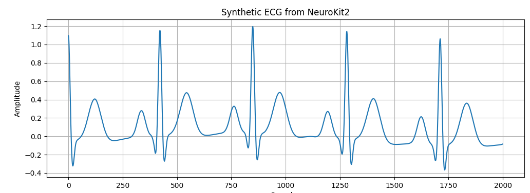
ecg[:2000]: plots only the first 2000 samples (~4 seconds) to zoom in. -
The plot shows ECG waveform: repeating cycles with P-wave, QRS complex, and T-wave.
-
figsize=(12,4): wide aspect ratio for clarity.
Step 3 – Frequency Analysis (FFT)
-
N = 5000(10 seconds × 500 samples/second).
-
FFT (Fast Fourier Transform) converts time-series → frequency domain.
-
np.fft.rfft→ computes FFT only for positive frequencies (saves space). -
np.fft.rfftfreq(N, 1/fs)→ generates the corresponding frequency bins (0 to Nyquist = fs/2 = 250 Hz).
Find Dominant Frequency
-
np.abs(fft_vals)→ magnitude spectrum (ignores phase). -
[1:]skips index0(DC component). -
np.argmax(...)→ index of the frequency with maximum amplitude. -
main_freq→ the dominant frequency (in Hz). -
main_bpm = main_freq * 60→ converts Hz to beats per minute.
Expected result:
-
Main frequency ≈ 1.17 Hz.
-
Heart rate ≈ 70 bpm (as set in the simulator).
Step 4 – Plot Frequency Spectrum
-
Plots the FFT spectrum: frequency on x-axis, magnitude on y-axis.
-
plt.xlim(0, 40)zooms in to 0–40 Hz (where heart-related frequencies live). -
You will see:
-
A main peak around 1.17 Hz → corresponds to heartbeat.
-
Smaller harmonics (multiples of 1.17 Hz) due to ECG waveform complexity.
-
|
1 2 3 4 5 6 7 8 9 10 11 12 13 14 15 16 17 18 19 20 21 22 23 24 25 |
# Frequency analysis fs = 500 # Sampling frequency in Hz N = len(ecg) # Number of samples # Apply FFT fft_vals = np.fft.rfft(ecg) # spectrum values fft_freqs = np.fft.rfftfreq(N, 1/fs) # corresponding frequencies # Find dominant frequency (skip DC at index 0) idx = np.argmax(np.abs(fft_vals[1:])) + 1 main_freq = fft_freqs[idx] # main frequency in Hz main_bpm = main_freq * 60 # convert to beats per minute print("Dominant frequency (Hz):", main_freq) print("Equivalent heart rate (bpm):", main_bpm) # Plot frequency spectrum plt.figure(figsize=(12,4)) plt.plot(fft_freqs, np.abs(fft_vals)) plt.title("Frequency spectrum of synthetic ECG") plt.xlabel("Frequency (Hz)") plt.ylabel("Magnitude") plt.grid(True) plt.xlim(0, 5) # ECG heartbeats usually below 5 Hz plt.show() |
Step 1 – Generate a Synthetic ECG
We use NeuroKit2’s ecg_simulate() function to create a clean ECG waveform.
import neurokit2 as nk

import matplotlib.pyplot as plt

import numpy as np
# Generate synthetic ECG (10 seconds, 500 Hz sampling rate, 70 bpm)
ecg = nk.ecg_simulate(duration=10, sampling_rate=500, heart_rate=70)
-
duration=10 → generate 10 seconds of signal
-
sampling_rate=500 → 500 samples per second
-
heart_rate=70 → target heart rate (70 beats per minute ≈ 1.17 Hz)
At this point, ecg is just a NumPy array with the amplitude values of the simulated ECG signal.
Step 2 – Plot the ECG
We can visualize the waveform and check its shape:
This plot shows the typical ECG waves (P, QRS, T complexes) repeated every heartbeat.
Step 3 – Frequency Analysis with FFT
To find the main repeating pattern in the ECG, we move to the frequency domain using the Fast Fourier Transform (FFT).
# Apply FFT
fft_vals = np.fft.rfft(ecg) # spectrum values
fft_freqs = np.fft.rfftfreq(N, 1/fs) # corresponding frequencies
# Find dominant frequency (skip DC at index 0)
idx = np.argmax(np.abs(fft_vals[1:])) + 1
main_freq = fft_freqs[idx] # main frequency in Hz
main_bpm = main_freq * 60 # convert to beats per minute
print("Dominant frequency (Hz):", main_freq)
print("Equivalent heart rate (bpm):", main_bpm)
# Plot frequency spectrum
plt.figure(figsize=(12,4))
plt.plot(fft_freqs, np.abs(fft_vals))
plt.title("Frequency spectrum of synthetic ECG")
plt.xlabel("Frequency (Hz)")
plt.ylabel("Magnitude")
plt.grid(True)
plt.xlim(0, 5) # ECG heartbeats usually below 5 Hz
plt.show()
Explanation
-
np.fft.rfft→ computes FFT for real-valued signals (positive frequencies only). -
np.fft.rfftfreq→ returns the frequency values for the spectrum. -
Dominant frequency is found by looking for the largest magnitude peak (excluding DC at 0 Hz).
-
Convert Hz → bpm by multiplying by 60.
For our simulation, the main frequency should be around 1.17 Hz, which equals 70 bpm—the same heart rate we set at the beginning.
Conclusion
With just a few lines of Python:
-
We generated a synthetic ECG signal.
-
We plotted and inspected the waveform.
-
We used FFT to extract its main repeating frequency and confirmed the heart rate.
This workflow demonstrates how to bridge between time domain (ECG waveform) and frequency domain (heart rate and rhythm analysis).
part 2 :
Find the repeated sequence
|
1 2 3 4 5 6 7 8 9 10 11 12 13 14 15 16 17 18 19 20 21 22 23 24 25 26 27 28 29 30 31 32 33 34 35 36 37 38 39 40 41 42 43 44 45 46 47 48 49 50 |
# -*- coding: utf-8 -*- """ Generate synthetic ECG with NeuroKit2 Shift data by 10 samples Plot waveform, frequency spectrum, and highlight repeated sequence (heartbeat) """ import neurokit2 as nk import matplotlib.pyplot as plt import numpy as np from scipy.signal import correlate # ========================================================= # 1. Generate synthetic ECG (10 seconds, 500 Hz, 70 bpm) # ========================================================= fs = 500 # sampling frequency ecg_full = nk.ecg_simulate(duration=10, sampling_rate=fs, heart_rate=70) # Shift data: start 10 samples later ecg = ecg_full[10:] print("Original length:", len(ecg_full), "Shifted length:", len(ecg)) # ========================================================= # 2. Detect repeated sequence (R-peaks) # ========================================================= signals, info = nk.ecg_peaks(ecg, sampling_rate=fs) rpeaks = info["ECG_R_Peaks"] # Take the first full heartbeat cycle (between first 2 R-peaks) start = rpeaks[0] end = rpeaks[1] heartbeat = ecg[start:end] # ========================================================= # 3. Plot original ECG (shifted) with extracted segment overlay # ========================================================= plt.figure(figsize=(12,4)) # Plot first 2000 samples of shifted ECG plt.plot(ecg[:2000], label="ECG Signal (shifted by 10 samples)") # Overlay extracted heartbeat on same scale, aligned at its true position plt.plot(range(start, end), heartbeat, color="red", linewidth=2, label="Extracted Heartbeat") plt.title("Synthetic ECG (Shifted by 10 Samples) with Highlighted Repeated Sequence") plt.xlabel("Samples") plt.ylabel("Amplitude") plt.legend() plt.grid(True) plt.show() |
line-by-line explanation of your “shifted ECG + repeated sequence overlay” script. I explain every function and parameter used.
-
Declares UTF-8 source encoding.
-
The docstring summarizes the script’s purpose.
-
neurokit2 as nk: toolkit for biosignal simulation/analysis (we’ll useecg_simulate,ecg_peaks). -
matplotlib.pyplot as plt: plotting API used for figures/axes (figure,plot,title, etc.). -
numpy as np: numerical arrays and slicing. -
scipy.signal.correlate: cross-correlation function (imported here but not used in this snippet; can be removed safely).
1) Generate ECG and shift by 10 samples
-
fs: sampling rate in Hz (samples per second). Here 500 Hz.
-
nk.ecg_simulate(...)creates a synthetic ECG as a 1-D NumPy array. -
Parameters:
-
duration=10: total signal duration in seconds → expected length ≈10 * fs = 5000samples. -
sampling_rate=fs: number of samples per second (here 500). -
heart_rate=70: target heart rate in bpm (beats per minute). 70 bpm ≈ 1.1667 Hz.
-
-
Return:
ecg_fullis the full ECG array (float values).
-
Slices the array starting at index 10, effectively shifting the signal by 10 samples (discarding the first 10 points).
-
New length is
len(ecg_full) - 10.
-
Prints the number of samples before/after shifting to confirm the 10-sample offset.
2) Detect the repeated sequence (R-peaks)
-
Detects R-peaks (the tall spikes in QRS complexes) in the shifted ECG.
-
Parameters:
-
ecg: the input ECG array (shifted). -
sampling_rate=fs: Hz; needed to set internal filter and timing scales.
-
-
Returns:
-
signals: dict/DataFrame with binary peak annotations (e.g.,ECG_R_Peaksseries). -
info: dictionary with indices of detected peaks and metadata. We’ll useinfo["ECG_R_Peaks"].
-
-
rpeaks: NumPy array of sample indices (integer positions inecg) where R-peaks occur. -
Note: these indices are relative to the shifted series (index 0 is
ecg_full[10]).
3) Extract one full heartbeat (the repeated sequence)
-
Takes the first two R-peaks to define one complete cardiac cycle (R-to-R interval).
-
start: sample index of first R-peak. -
end: sample index of next R-peak. -
Assumes at least two peaks were found; for safety in production code, check
len(rpeaks) >= 2.
-
Slices the ECG between
start(inclusive) andend(exclusive). -
heartbeatis a 1-cycle waveform (the repeated sequence you want to show).
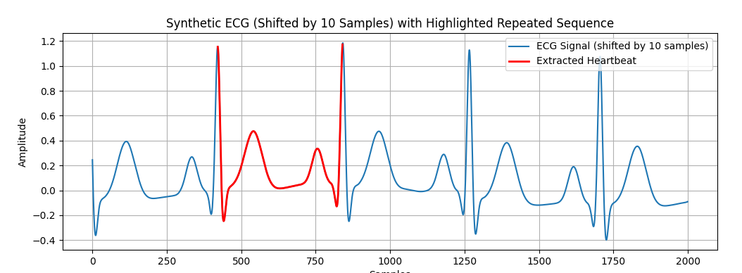
4) Plot the shifted ECG and overlay the extracted heartbeat
-
Creates a new figure.
-
Parameter:
-
figsize=(12,4): width 12 inches, height 4 inches.
-
-
Plots the first 2000 samples (~4 seconds at 500 Hz) of the shifted ECG.
-
Parameter:
-
label="...": legend entry for this line.
-
-
The x-axis here is sample index
0..1999(in the shifted reference frame).
-
Overlays the extracted heartbeat on the same axes and scale:
-
range(start, end): x-coordinates aligned to the original sample positions within the shifted ECG.
This ensures the segment appears exactly where it occurs in the larger signal. -
heartbeat: y-values for that segment.
-
-
Parameters:
-
color="red": draw the overlay in red. -
linewidth=2: slightly thicker line for visibility. -
label="...": legend entry.
-
-
title,xlabel,ylabel: annotate the plot. -
plt.legend(): shows labels fromlabel=inplot. -
plt.grid(True): turn on grid lines. -
plt.show(): renders the figure.
Notes and best practices
-
If
ecg_peakssometimes misses peaks (rare with clean synthetic data), you can fine-tune withmethodand cleaning parameters in NeuroKit2 (e.g.,nk.ecg_cleanbefore peak detection). -
For robustness, check
len(rpeaks) >= 2before slicingheartbeat. -
The overlay uses true indices (
range(start, end)), so the repeated sequence is displayed on the same scale and at the exact location inside the original graph, as requested. -
Because you shifted by 10 samples, all indices and plots refer to the shifted signal; the absolute time offset is
10 / fsseconds.
|
1 2 3 4 5 6 7 8 9 10 11 12 13 14 15 16 17 18 19 20 21 22 23 24 25 26 27 28 29 30 31 32 33 34 35 36 37 38 39 40 41 42 43 44 45 46 47 48 49 50 51 52 53 54 55 56 57 58 59 60 61 62 63 64 65 66 67 68 69 70 71 72 73 74 75 76 77 78 79 80 81 82 83 84 85 86 87 88 89 90 91 92 93 94 95 96 97 98 99 100 101 102 103 104 105 106 107 108 109 110 111 112 113 114 115 116 117 118 119 120 121 122 |
# -*- coding: utf-8 -*- """ Created on Sat Sep 27 05:29:39 2025 @author: dev66 """ # -*- coding: utf-8 -*- """ Generate synthetic ECG with NeuroKit2 Shift data by 10 samples Add four noise cases: random, sinusoidal drift, hybrid, and repeated periodic noise Plot results and highlight repeated sequence """ import neurokit2 as nk import matplotlib.pyplot as plt import numpy as np # ========================================================= # 1. Generate synthetic ECG (10 seconds, 500 Hz, 70 bpm) # ========================================================= fs = 500 # sampling frequency ecg_full = nk.ecg_simulate(duration=10, sampling_rate=fs, heart_rate=70) # Shift the signal by 10 samples ecg = ecg_full[10:] t = np.arange(len(ecg)) / fs # time axis in seconds # ========================================================= # 2. Define noise signals # ========================================================= rand_noise = 0.1 * np.random.randn(len(ecg)) # Random Gaussian noise vig_noise = 0.3 * np.sin(2 * np.pi * 0.5 * t) # Sinusoidal drift (0.5 Hz) hybrid_noise = rand_noise + vig_noise # Combination repeated_noise = 0.15 * np.sin(2 * np.pi * 50 * t) # Repeated interference (50 Hz) # ========================================================= # 3. Create noisy ECG variants # ========================================================= ecg_random = ecg + rand_noise ecg_sinus = ecg + vig_noise ecg_hybrid = ecg + hybrid_noise ecg_repeated = ecg + repeated_noise # ========================================================= # 4. Function to extract first repeated heartbeat # ========================================================= def extract_heartbeat(signal, fs): signals, info = nk.ecg_peaks(signal, sampling_rate=fs) rpeaks = info["ECG_R_Peaks"] if len(rpeaks) >= 2: start, end = rpeaks[0], rpeaks[1] return start, end, signal[start:end] else: return None, None, None # Extract heartbeats s0, e0, beat_clean = extract_heartbeat(ecg, fs) s1, e1, beat_random = extract_heartbeat(ecg_random, fs) s2, e2, beat_sinus = extract_heartbeat(ecg_sinus, fs) s3, e3, beat_hybrid = extract_heartbeat(ecg_hybrid, fs) s4, e4, beat_repeated = extract_heartbeat(ecg_repeated, fs) # ========================================================= # 5. Plot comparisons with repeated sequence overlay # ========================================================= plt.figure(figsize=(14,12)) # Clean ECG plt.subplot(5,1,1) plt.plot(ecg[:2000], label="Clean ECG") if beat_clean is not None: plt.plot(range(s0, e0), beat_clean, color="red", linewidth=2, label="Repeated sequence") plt.title("Clean Synthetic ECG (first 2000 samples)") plt.ylabel("Amplitude") plt.legend() plt.grid(True) # ECG + random noise plt.subplot(5,1,2) plt.plot(ecg_random[:2000], label="ECG + Random Noise") if beat_random is not None: plt.plot(range(s1, e1), beat_random, color="red", linewidth=2, label="Repeated sequence") plt.title("ECG + Random Gaussian Noise") plt.ylabel("Amplitude") plt.legend() plt.grid(True) # ECG + sinusoidal drift plt.subplot(5,1,3) plt.plot(ecg_sinus[:2000], label="ECG + Sinusoidal Drift") if beat_sinus is not None: plt.plot(range(s2, e2), beat_sinus, color="red", linewidth=2, label="Repeated sequence") plt.title("ECG + Sinusoidal Drift (0.5 Hz)") plt.ylabel("Amplitude") plt.legend() plt.grid(True) # ECG + hybrid noise plt.subplot(5,1,4) plt.plot(ecg_hybrid[:2000], label="ECG + Hybrid Noise") if beat_hybrid is not None: plt.plot(range(s3, e3), beat_hybrid, color="red", linewidth=2, label="Repeated sequence") plt.title("ECG + Hybrid Noise (Random + Sinusoidal)") plt.ylabel("Amplitude") plt.legend() plt.grid(True) # ECG + repeated periodic noise plt.subplot(5,1,5) plt.plot(ecg_repeated[:2000], label="ECG + Repeated Noise") if beat_repeated is not None: plt.plot(range(s4, e4), beat_repeated, color="red", linewidth=2, label="Repeated sequence") plt.title("ECG + Repeated Noise (50 Hz interference)") plt.xlabel("Samples") plt.ylabel("Amplitude") plt.legend() plt.grid(True) plt.tight_layout() plt.show() |
Explanation of Each Section
1. ECG Generation
-
duration=10→ create 10 seconds of ECG data. -
sampling_rate=500→ 500 samples per second. -
heart_rate=70→ simulate a heart rate of 70 beats per minute.
We then shift the signal by 10 samples:
2. Adding Noise
We define four types of noise:
-
Random Gaussian Noise:
Simulates random electrical fluctuations.
-
Sinusoidal Drift:
Low-frequency baseline wander (e.g., breathing, electrode motion).
-
Hybrid Noise:
Combination of the two above.
-
Repeated Noise:
Simulates 50 Hz periodic interference (like mains power hum).
3. Create Noisy ECG Variants
Each noisy version is created by adding the noise to the clean ECG:
4. Extract the Repeated Sequence
We use NeuroKit2’s ecg_peaks to detect R-peaks:
-
The first two R-peaks define one heartbeat cycle:
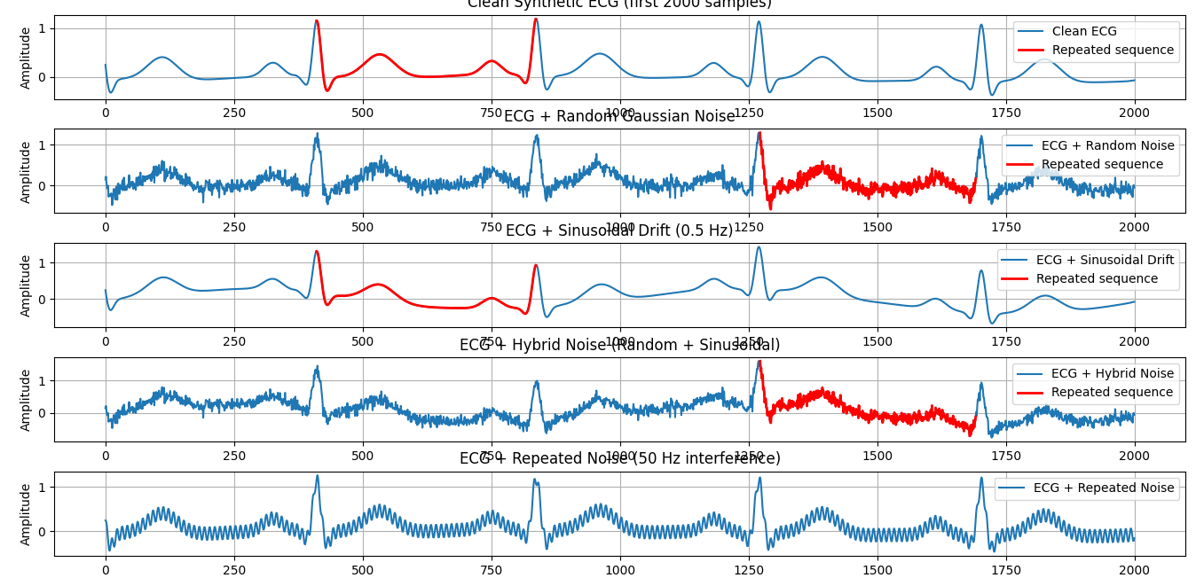
5. Plot Results
We plot 2000 samples (~4 seconds) for each case:
-
Clean ECG
-
ECG + random noise
-
ECG + sinusoidal drift
-
ECG + hybrid noise
-
ECG + repeated noise
On each graph:
-
The full ECG is in blue.
-
The extracted repeated heartbeat cycle is overlaid in red.
Conclusion
This script demonstrates how:
-
Noise affects ECG signals differently.
-
Even with noise, repeated heartbeat cycles can be extracted using R-peak detection.
-
You can simulate realistic ECG scenarios for testing signal-processing algorithms.