A.I Predict Iris flower species (Setosa, Versicolor, Virginica).
 Iris is a flowering plant genus of 310 accepted species[1] with showy flowers. As well as being the scientific name, iris is also widely used as a common name for all Iris species, as well as some belonging to other closely related genera. A common name for some species is flags, while the plants of the subgenus Scorpiris are widely known as junos, particularly in horticulture. It is a popular garden flower
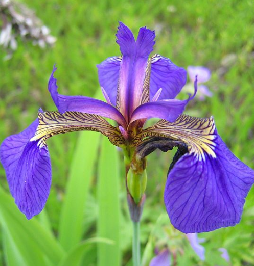
Setosa
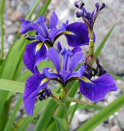
Versicolor
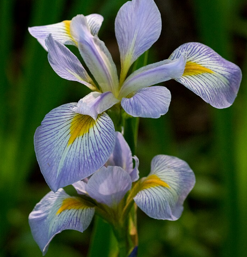
Virginica
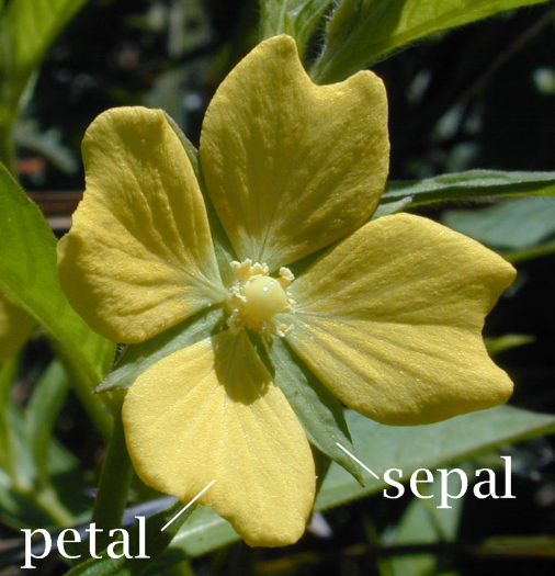
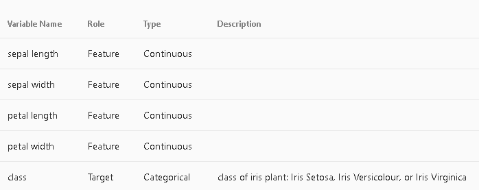
: Variable table
4.9,3.0,1.4,0.2,Iris-setosa
4.7,3.2,1.3,0.2,Iris-setosa
…
6.4,3.2,4.5,1.5,Iris-versicolor
6.9,3.1,4.9,1.5,Iris-versicolor
5.8,2.7,5.1,1.9,Iris-virginica
7.1,3.0,5.9,2.1,Iris-virginica
https://archive.ics.uci.edu/dataset/53/iris
What do the instances in this dataset represent?
Additional Information
download the file iris-flower-p
|
1 2 3 4 5 6 7 8 9 10 11 12 13 14 15 16 17 18 19 20 21 22 23 24 25 26 27 28 29 30 31 32 33 34 35 36 37 38 39 40 41 42 43 44 45 46 47 48 49 50 51 52 53 54 55 56 57 58 59 60 61 62 63 64 65 66 67 68 69 70 71 72 73 74 75 76 77 78 79 80 81 82 83 84 85 86 87 88 89 90 91 92 93 94 95 96 97 98 99 100 101 102 103 104 105 106 107 108 109 110 111 112 113 114 115 116 117 118 119 120 121 122 123 124 125 126 127 128 129 130 131 132 133 134 135 136 |
# -*- coding: utf-8 -*- """ Iris Flower Classification with ANN Author: Example Dataset: d:\temp\iris-flower-p.csv """ import pandas as pd import numpy as np import matplotlib.pyplot as plt from sklearn.model_selection import train_test_split from sklearn.preprocessing import LabelEncoder, StandardScaler from tensorflow import keras from tensorflow.keras import layers # ====================================================== # 1) Load dataset # "skiprows=1" ensures first row (column headers from Excel-like export) is ignored # ====================================================== file_path = r"d:\temp\iris-flower-p.csv" df = pd.read_csv(file_path, skiprows=1, header=None) # Rename columns manually (since we skipped header row) df.columns = ["sepal length", "sepal width", "petal length", "petal width", "class"] print("=== Dataset Summary ===") print("Number of records:", len(df)) print("Number of features:", df.shape[1]-1) # exclude 'class' print("\nClass distribution:") print(df["class"].value_counts()) # ====================================================== # 2) Correlation matrix (text only) # ====================================================== print("\n=== Correlation Matrix ===") corr = df.drop("class", axis=1).corr() print(corr) # ====================================================== # 3) Split features (X) and labels (y) # ====================================================== X = df.drop("class", axis=1).values y = df["class"].values # Encode labels into numbers encoder = LabelEncoder() y_encoded = encoder.fit_transform(y) # ====================================================== # 4) Scale features # ====================================================== scaler = StandardScaler() X_scaled = scaler.fit_transform(X) print("\n=== Data before flattening ===") print("Shape:", X_scaled.shape) # e.g., (150,4) print(X_scaled[:5]) # Flatten: in ANN we want input as a vector X_flat = X_scaled.reshape(X_scaled.shape[0], -1) print("\n=== Data after flattening ===") print("Shape:", X_flat.shape) print(X_flat[:5]) # ====================================================== # 5) Train-test split # ====================================================== X_train, X_val, y_train, y_val = train_test_split( X_flat, y_encoded, test_size=0.2, random_state=42, stratify=y_encoded ) # ====================================================== # 6) Build ANN model # ====================================================== num_classes = len(np.unique(y_encoded)) model = keras.Sequential([ layers.Input(shape=(X_flat.shape[1],)), # input layer layers.Dense(16, activation="relu"), # hidden layer layers.Dense(8, activation="relu"), # hidden layer layers.Dense(num_classes, activation="softmax") # output layer ]) model.compile( optimizer="adam", loss="sparse_categorical_crossentropy", metrics=["accuracy"] ) print("\n=== Model Summary ===") model.summary() # ====================================================== # 7) Train the model # ====================================================== history = model.fit( X_train, y_train, validation_data=(X_val, y_val), epochs=90, batch_size=8, verbose=1 ) # ====================================================== # 8) Save model # ====================================================== model_file = r"d:\temp\iris_ann_model.h5" print("\n=== Model Saved ===") print(f"Model file: {model_file}\n") model.save(model_file) # ====================================================== # 9) Show training history # ====================================================== plt.figure(figsize=(10,4)) # Plot loss plt.subplot(1,2,1) plt.plot(history.history["loss"], label="Train Loss") plt.plot(history.history["val_loss"], label="Validation Loss") plt.xlabel("Epochs") plt.ylabel("Loss") plt.title("Loss over Epochs") plt.legend() # Plot accuracy plt.subplot(1,2,2) plt.plot(history.history["accuracy"], label="Train Accuracy") plt.plot(history.history["val_accuracy"], label="Validation Accuracy") plt.xlabel("Epochs") plt.ylabel("Accuracy") plt.title("Accuracy over Epochs") plt.legend() plt.show() |
=== Model Saved ===
Model file: d:\temp\iris_ann_model.h5

Iris Flower Classification with an Artificial Neural Network (ANN)
This program demonstrates how to build a simple Artificial Neural Network (ANN) using TensorFlow and Keras to classify iris flowers based on their features.
The dataset is stored in a CSV file (d:\temp\iris-flower-p.csv) and contains sepal length, sepal width, petal length, petal width, and the class (flower type).
Step 1: Importing the Required Libraries
-
pandas: to load and work with the CSV file as a table.
-
numpy: to handle numbers and arrays.
-
matplotlib.pyplot: to create graphs.
-
train_test_split: to split the dataset into training and validation sets.
-
LabelEncoder: to convert text labels (flower names) into numbers.
-
StandardScaler: to scale features for better ANN training.
-
keras and layers: to build the ANN itself.
Step 2: Loading the Dataset
-
skiprows=1: skips the first row in case it has extra information. -
header=None: prevents pandas from treating the first row as column names. -
The columns are then renamed manually for clarity.
Step 3: Dataset Summary
-
len(df): number of rows (records). -
df.shape[1]-1: number of features, excluding the class column. -
value_counts(): shows how many examples exist for each flower type.
Step 4: Correlation Matrix
-
Drops the class column (because it’s text).
-
.corr(): calculates how numeric features are related. For example, petal length and petal width are strongly correlated.
Step 5: Preparing Features and Labels
-
X: the numeric data (inputs for the model). -
y: the flower type (target output).
Step 6: Encoding the Labels
-
Converts class names into numbers: Setosa → 0, Versicolor → 1, Virginica → 2.
Step 7: Scaling the Features
-
Scales all features so they are on a similar range (mean 0, standard deviation 1).
-
This helps the neural network learn faster and more reliably.
Step 8: Flattening the Features
-
Ensures the input data is in the correct shape: one row per flower, one column per feature.
-
Neural networks expect flat (one-dimensional) inputs, not multi-dimensional tables.
Step 9: Splitting into Training and Validation Sets
-
test_size=0.2: 20% of the dataset is reserved for validation. -
random_state=42: ensures the split is always the same when rerunning the code. -
stratify=y_encoded: makes sure each set has the same class proportions.
Step 10: Building the ANN Model
-
Input layer: accepts the four features.
-
Dense(16, activation="relu"): first hidden layer with 16 neurons.
-
Dense(8, activation="relu"): second hidden layer with 8 neurons.
-
Dense(num_classes, activation="softmax"): output layer with one neuron per class, using softmax to output probabilities.
Step 11: Compiling the Model
-
optimizer="adam": adjusts weights during training.
-
loss="sparse_categorical_crossentropy": correct loss for multi-class problems with integer labels.
-
metrics=["accuracy"]: tracks accuracy during training.
Step 12: Training the Model
-
epochs=90: the network sees the entire dataset 90 times. -
batch_size=8: processes 8 samples at a time before updating weights. -
validation_data: evaluates performance on unseen validation data. -
verbose=1: prints training progress.
Step 13: Saving the Model
-
Saves the trained model to a file called
iris_ann_model.h5. -
The model can later be reloaded to make predictions without retraining.
Step 14: Visualizing Training History
-
Creates two plots:
-
Loss vs Epochs: shows how the error decreases.
-
Accuracy vs Epochs: shows how prediction accuracy improves.
-
-
These plots help confirm whether the model is learning effectively.
Key Parameters Recap
-
skiprows=1: skips the first row in the CSV file. -
train_test_split(test_size=0.2, random_state=42, stratify=y): controls dataset splitting. -
Dense(units, activation): defines each layer of the ANN. -
compile(optimizer, loss, metrics): defines how the model learns. -
fit(epochs, batch_size, validation_data): controls the training process.
This program demonstrates the full workflow of building an ANN:
loading the data, preparing it, building a network, training it, saving it, and finally visualizing the training progress.
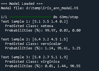
Prediction :
Perfect. Let’s create a prediction script that:
-
Loads the saved model (
iris_ann_model.h5). -
Defines a few test flower measurements:
-
[5.1, 3.5, 1.4, 0.2] -
[6.4, 3.2, 4.5, 1.5] -
[5.8, 2.7, 5.1, 1.9]
-
-
Preprocesses them the same way as during training (StandardScaler).
-
Predicts class probabilities (percentages).
-
Prints the predicted class name and confidence %.
|
1 2 3 4 5 6 7 8 9 10 11 12 13 14 15 16 17 18 19 20 21 22 23 24 25 26 27 28 29 30 31 32 33 34 35 36 37 38 39 40 41 42 43 44 45 46 47 48 49 50 51 52 53 54 55 56 57 58 59 60 61 62 63 64 65 66 67 68 69 70 71 72 73 74 |
# -*- coding: utf-8 -*- """ Test predictions with trained Iris ANN model Dataset: d:\temp\iris-flower-p.csv Model: d:\temp\iris_ann_model.h5 """ import pandas as pd import numpy as np from sklearn.preprocessing import LabelEncoder, StandardScaler from tensorflow import keras # ====================================================== # 1) Load dataset again (to rebuild encoder + scaler) # ====================================================== file_path = r"d:\temp\iris-flower-p.csv" df = pd.read_csv(file_path, skiprows=1, header=None) # Rename columns df.columns = ["sepal length", "sepal width", "petal length", "petal width", "class"] # Features and labels X = df.drop("class", axis=1).values y = df["class"].values # Encode labels encoder = LabelEncoder() y_encoded = encoder.fit_transform(y) # Scale features (fit on training data) scaler = StandardScaler() scaler.fit(X) # ====================================================== # 2) Load trained model # ====================================================== model_file = r"d:\temp\iris_ann_model.h5" model = keras.models.load_model(model_file) print("\n=== Model Loaded ===") print(f"Model file: {model_file}\n") # ====================================================== # 3) Define test samples # ====================================================== test_samples = np.array([ [5.1, 3.5, 1.4, 0.2], # Expected: Setosa [6.4, 3.2, 4.5, 1.5], # Expected: Versicolor [5.8, 2.7, 5.1, 1.9] # Expected: Virginica ]) # Scale samples using the same scaler test_scaled = scaler.transform(test_samples) # ====================================================== # 4) Make predictions # ====================================================== pred_probs = model.predict(test_scaled) pred_classes = np.argmax(pred_probs, axis=1) # ====================================================== # 5) Print results # ====================================================== for i, sample in enumerate(test_samples): class_idx = pred_classes[i] class_name = encoder.inverse_transform([class_idx])[0] probabilities = pred_probs[i] * 100 # convert to percent # Format probabilities as floats with 2 decimals probs_str = ", ".join([f"{p:.2f}" for p in probabilities]) print(f"Test Sample {i+1}: {sample}") print(f" Predicted Class: {class_name}") print(f" Probabilities (%): {probs_str}") print() |